Mixture modeling of paralog K_S distributions

The interpretation of mixed paralog–ortholog K_S distributions is sometimes challenging due to the fact that paralog WGD peaks are often not clearly distinguishable because of progressive WGD signal erosion over time and potential overlapping of multiple peaks from successive WGDs. In order to more objectively define the K_S age of potential WGD peaks, a clustering feature based on mixture modeling has been implemented in ksrates.

Three methods are available: anchor K_S clustering, exponential-lognormal mixture modeling and lognormal-only mixture modeling. A short overview can be found below. For an extended description of these methods, please refer to the Supplementary Materials of the preprint.

Warning

Please be aware that mixture modeling results on K_S distributions should be interpreted cautiously because mixture models tend to overestimate the number of components present in the target K_S distribution and hence the number of WGDs.

Settings in the ksrates configuration files determine which methods are applied and which are not (see also sections ksrates configuration file and Expert configuration file):

• If collinearity analysis is selected in the ksrates configuration file (collinearity = yes), the default method performed is a clustering based on the anchor pair K_S values in collinear segment pairs.

• Otherwise (collinearity = no and paranome = yes), the default method performed is exponential-lognormal mixture modeling of the whole-paranome K_S distribution.

• Lognormal-only mixture modeling can be turned on for comparison. It is never applied by default, since it is more prone to produce spurious peaks.

The execution of non-default methods according to the scheme in the table below can be turned on with a setting in the expert configuration file. For example, when both collinearity and paranome analyses are selected (last column), only the anchor K_S clustering is perfomed by default and all the other methods can be turned on optionally.

Default methods are marked by ✓, while optional methods are marked by (✓).

Method	Collinearity-only	Paranome-only	Collinearity and paranome
Anchor KS clustering	✓		✓
Exponential-lognormal mixture model		✓	(✓)
Lognormal mixture model on anchor pairs	(✓)		(✓)
Lognormal mixture model on paranome		(✓)	(✓)

Anchor K_S clustering

A clustering approach is used in order to classify anchor pair K_S values into groups that potentially stem from different WGDs in the ancestry of the focal species. The approach does not cluster the anchor pair K_S values directly, but instead uses lognormal mixture modeling to cluster median K_S values for the collinear segment pairs, i.e. pairs of sequence regions with conserved gene content and order, that the anchor pairs reside on. Segment pairs originated by the same WGD are likely to share a similar K_S age and to fall into the same cluster.

Such segment-pair medians are then clustered through lognormal mixture modeling. In order to obtain the clusters of the original anchor K_S data, each median K_S value is replaced by the K_S list of the segment pair. Anchor K_S clusters for which a link to a real WGD event is ambiguous or unlikely are removed from the dataset (i.e. small, flat or old clusters).

Exponential-lognormal mixture model

ksrates implements a custom exponential-lognormal mixture model (ELMM) algorithm for analyzing whole-paranome K_S distributions. The exponential component is used to model the L-shaped background of a whole-paranome K_S distribution generated by small-scale duplications, while one or more lognormal components are used to model potential WGD peaks.

Since adequate initialization of the component parameters is crucial for obtaining decent mixture modeling results, ksrates uses three different initialization approaches and ultimately chooses the best one based on the Bayesian Information Criterion (BIC):

• Data-driven initialization, which infers component parameters from the shape of the K_S distribution. The exponential component is initialized to match the height of the left boundary of the distribution, while each lognormal component is initialized in correspondence of a peak.

• Initialization with random component parameters, by default with two to five random components.

• Hybrid initialization, where one random lognormal component is added to the data-driven initialized components in the attempt to compensate for possible overlooked signals.

In all three strategies, an extra “buffer” lognormal component is initialized by default at the right boundary of the K_S range to avoid that other components stretch towards higher values in an attempt to fit the hard-to-fit distribution tail.

Data output file format

Among its outputs (for a complete list see section Output files and directory organization), the ELMM produces a tabular (TSV) file and a text file where parameters and fitting results are stored:

• elmm_species_parameters.tsv:

  • The model initialization approach is stored in column 1 Model according to a numerical code (1: data-driven, 2: hybrid data-driven plus a random lognormal component, 3: random initialization with exponential component and one lognormal component, 4: random initialization with exponential component and two lognormal components; higher numbers feature random initialization with exponential component and increasing number of lognormal components).

  • The initialization round is stored in column 2 Initialization. By default each model type (except type 1) is initialized and fitted 10 times, so this column shows numbers from 1 to 10.

  • The BIC and loglikelihood scores for the fitted model are stored in columns 3 BIC and 4 Loglikelihood.

  • The number of algorithm iterations needed to reach convergence is stored in column 5 Convergence. If greater than (by default) 600 iterations would be needed, convergence is not reached and the cell will show NA.

  • The fitted exponential rate parameter and its component weight are stored in columns 6 Exponential_Rate and 7 Exponential_Weight.

  • The mean, standard deviation and weight of the fitted Normal components used to define the correspondent lognormal components are stored in columns 8 to 10: Normal_Mean, Normal_SD and Normal_Weight. When there are multiple lognormal components, the data for each of them are stored in a separate row (the number of rows for each model and initialization is thus equal to the number of lognormal components).

This file section shows the result for the first initalization of model 5: each row stores the same data for the exponential component plus the data for one of the three lognormal components.

• elmm_species_parameters.txt reports the results in a more descriptive and easy-to-read logging format.

Lognormal mixture model

Logormal mixture modeling (LMM) makes use of only lognormal components and is optionally available both for whole-paranome and anchor pair K_S distributions using a setting in the expert configuration file.

The lognormal components are initialized through k-means and fitted by default with two to five components. For each number of components the mixture model is initialized multiple times and the best fit is chosen according to the largest log-likelihood. Among the resulting four models (one for each number of components), the best fitting model is taken to be the one with the lowest BIC score.

Warning

LMM is more prone than ELMM to detect spurious peaks in the left side of the whole-paranome K_S distribution because it is less suitable to fit the small-scale duplication background.

Data output file format

Among its outputs (for a complete list see section Output files and directory organization), the LMM produces tabular (TSV) files and text files where parameters and fitting results are stored:

• lmm_species_parameters_paranome.tsv and lmm_species_parameters_anchors.tsv:

  • The model type is stored in column 1 Model according to a numerical code (1: one lognormal component, 2: two lognormal components, 3: three lognormal components; and so on).

  • The BIC and loglikelihood scores for the fitted model are stored in columns 2 BIC and 3 Loglikelihood

  • The number of algorithm iterations needed to reach convergence is stored in column 4 Convergence. If greater than (by default) 600 iterations would be needed, convergence is not reached and the cell will show NA.

  • The mean, standard deviation and weight of the fitted Normal components used to define the correspondent lognormal components are stored in columns 5 to 7: Normal_Mean, Normal_SD and Normal_Weight. When there are multiple lognormal components, the data for each of them are stored in a separate row (the number of rows per model is thus equal to the number of components).

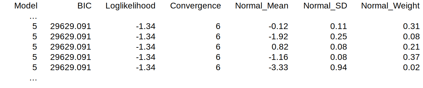
This file section shows the result for model 5: each row stores the data for one of the five lognormal components.

• lmm_species_parameters_paranome.txt and lmm_species_parameters_anchors.txt collect the model results in a more descriptive and easy-to-read logging format.